Heavy buildings or structures make the ground compress a little over time due to their weight. This compression of soil is known as the Settlement of soil.

 

 

Total settlement of the soil has primarily three components.

1. Immediate Settlement

2. Consolidation Settlement or Primary Consolidation

3. Creep Settlement or Secondary Consolidation

 

The Total Settlement of soil is the sum of all three factors

 

 

Consolidation Settlement is the most dominant factor of the total settlement. It refers to the settlement of soil that occurs because applied load causes the rearrangement of soil particles and dissipation of excess pore water pressure in saturated soils. We have learned all this in our previous post.

 

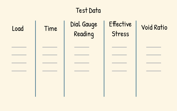
To estimate the amount of settlement and rate of consolidation we perform consolidation test on soil sample in laboratory. The consolidation test also helps determine various soil properties of clay relevant to consolidation, such as the permeability, swelling behaviour of soil and coefficient of consolidation.

 

We have discussed part of the consolidation test in our previous post where we plotted a time-settlement curve under a single load. Now we’ll be loading the soil specimen with higher load incrementally in steps.

 

The test is carried out in a device called an Oedometer or a Consolidometer. This device has two main components: a container for the soil sample, known as the consolidation cell and a loading system that applies pressure.

 

 

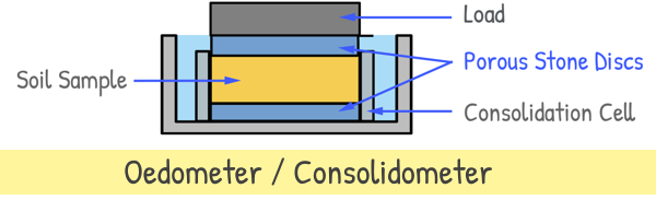
Top and bottom of the sample are equipped with porous stone discs. These discs enable two-way vertical drainage, allowing water to flow freely in and out of the soil.

 

The soil sample is carefully placed inside the consolidation cell. Then a load in placed on top of the cell. The soil is allowed to consolidate (settle) until practically no further compression occurs. This ensures all excess water pressure within the pores is entirely dissipated. Typically, the load is maintained for a full day (that is 24 hours).

 

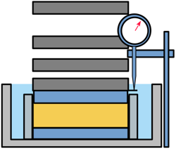A dial gauge is used to measure the deformation of the specimen in the vertical direction. The dial gauge readings are recorded at various time intervals after applying the load. Last reading is taken at 24 hours.

Then more load is applied on the soil and again soil is allowed to consolidate and dial gauge readings are noted.

Similarly load is gradually increased in steps and readings are noted.

 

After the soil has fully settled under the final load increment, we'll gradually reduce the load in two or three steps. After each unloading the sample is allowed to swell and expand. We note down the readings after each unloading to track the amount of expansion.

Finally we place the sample in an oven for drying to determine the weight of solids and the final water content.

 

Our objective is to observe and determine the compression of soil that is taking place under the applied load. For the purpose we use void ratio as a measure to determine the amount of compression of soil because It is primarily the voids that decrease in size, when a load is applied, leading to soil compression.

Therefore, we aim to determine how the void ratio changes with the application of load. And for that we plot a graph between void ratio and effective stress using the data obtained from the test. But the problem is, test data does not give us directly the effective stress and void ratio for each load increment.

 

 

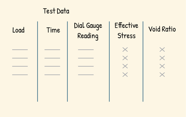
Effective Stress is just the pressure experienced by soil particles. Which is different from the pressure due to load on the surface of soil, as soil, including soil particles, also contains air and water. They also support part of the load. Effective Stress has been described in detail in our previous post.

So, to calculate effective stress we use a known relationship between effective stress, total stress and pore water pressure.

σ' = σ – u

 

σ' = effective stress

σ = Total Stress and that can be calculated from the applied load and the area of the soil sample being tested

u = Pore water pressure and it is usually measured directly using a piezometer installed within the soil sample during the consolidation test

So with these known, we can calculate effective stress for each data point in the table.

 

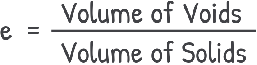
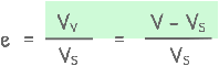
Now we come to the void ratio. Void ratio, represented by “e”, of a soil sample is the ratio of the space occupied by the voids i.e. volume of voids to the space occupied by the solids i.e. volume of solids.

 

To compute final void ratio after each load increment, one of the two methods is usually adopted :

1. Height of Solids Method and

2. Change in Void Ratio Method

 

Height of Solids Method

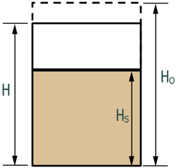In this method the soil is considered as 2 phase system. Here volume and height of the sample at the beginning was V₀ and H₀ respectively. Height of solids is H_s. Lets say after a few load increments its volume and height has become V and H respectively but height of the solids will remain the same. Now using the 2 phase diagram we can write height of solids as volume of solids divided by area of the sample.

 

Using a known relationship :

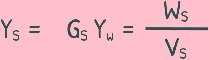
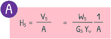
volume of solids can also be written as weight of solids divided by specific gravity of solids and unit weight of water.

 

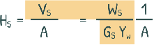
In the equation W_S, weight of solids can be determined by oven drying the sample. Specific Gravity of Solids can be obtained via pycnometer test or other standard methods. The Unit weight of water is a known constant value. Therefore, all the quantities in this equation are known, so we can calculate height of solids. We keep this equation and name it as equation number A.

 

Now we know the void ratio is volume of voids divided by volume of solids

 

Volume of voids can be written as total volume of soil minus volume of solids.

 

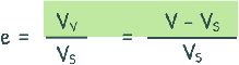
Volume of sample can be written as area of sample multiplied by height of sample and volume of solids can be written as area of sample multiplied by height of solids.

 

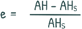
by simplifying we obtain void ratio of the soil sample

 

In this equation we have already calculated the

H_S = Height of solids by equation number A and it is going to remain constant

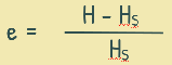
H = Height of the soil sample after load application when pore pressure dissipated and soil has reached equilibrium. It can be given as initial height of the specimen plus minus change in its height due to either swelling or compression.

 

H₀ = Initial height of the specimen at the beginning of test

ΔH = is the change in thickness of sample under the load increment which can be read by dial gauge

 

With this, now we can calculate void ratios for all the load increments.

 

 

the other method of calculating the void ratio for different load increments is

Change in Void Ratio Method

In this method the void ratio of the saturated soil at the end of the test is calculated from a known relationship

Se = wG

 

here soil is saturated so degree of saturation is 1 so we can write

 

w_f is the final water content at the end of the test which was obtained via oven drying method. Hence we can calculate the final void ratio of the soil sample using this equation.

 

And the void ratio at the end of each loading increment can be determined from definition of void ratio

 

we can write volume of voids as total volume of sample minus volume of solids.

 

and it can be simplified to this

 

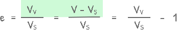
and after a little re-arrangement we receive this

V = V_s (1 + e )

 

Now volume of sample can be written as area of sample which is constant multiplied by height of sample after it has reached equilibrium

note this equation as equation number B. Only two quantities are variable here, so by partial differentiation of this we get this.

A dH = Vs de

 

now using the above equation B, we can write it as this

 

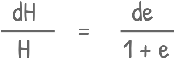
and after a little rearrangement we get this.

 

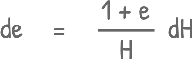
and for a small change we can write it as this also

 

This equation describes that when a soil sample is compressed under a load, change in its void ratio Δe and change in its height ΔH occurs. The sample attains new height H and void ratio e. Hence we can also write them as e_f and H_f representing final void ratio and final height of the sample after consolidation.

 

Since the final void ratio ef and the sample height after consolidation at different loadings are known, we can calculate the change in void ratio (Δe) for each load increment directly using the equation by working backwards from the known value of void ratio e_f.

 

 

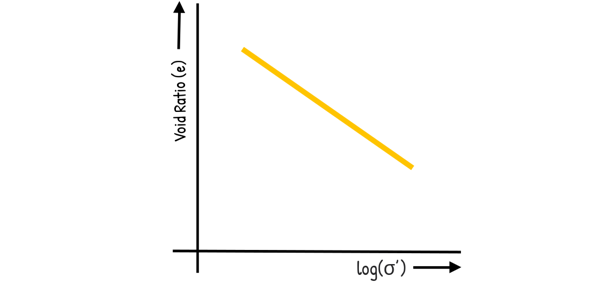
With that, we now have both effective stress (σ₁, σ₂, σ₃ etc.) and final void ratio (e_f1 e_f2 e_f3… etc.) data at different loadings for our consolidation test we can now plot the graph between them.

 

 

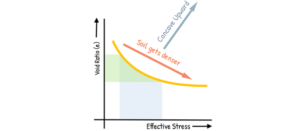
We can see the curve generally has a downward trend, indicating that as the effective stress, that is pressure on the soil particles, increases, the void ratio decreases. This signifies the soil is compacting due to the applied pressure and becoming denser.

This curve has concavity upward and the slope of the curve is not constant. It is steeper initially and becomes flatter as effective stress increases. This indicates that rate of void ratio reduction decreases as the stress on soil particles increases.

If the soil is subjected to a certain stress increment, say Δσ, it will undergo some decrease in void ratio lets say equal to Δe₁. It indicates there is some degree of densification in soil. Now If the soil is subjected to the same magnitude of stress increment Δσ again, this time, the reduction in void ratio will not be equal to Δe₁, but it will be less than Δe₁, say it is Δe₂.

 

 

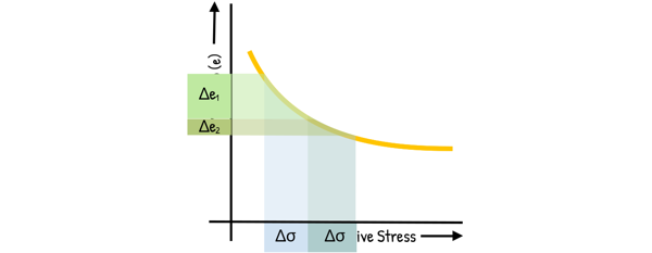
This demonstrates that as effective stress increases, the compressibility of the soil decreases. This relationship is quantified by the Coefficient of Compressibility, a_v, which defines the slope of the void ratio – effective stress curve. For a small stress increment the curve can be approximated as straight line and Coefficient of Compressibility is defined as the decrease in void ratio per unit increase in effective stress.

 

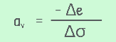
From this relationship and by looking at the graph we can say, the coefficient of compressibility decreases as effective stress increases. In simpler words soil becomes hard and less compressible as the effective stress is increased.

Also as the effective stress increases, the void ratio decreases, hence the change in void ratio is negative. But the coefficient of compressibility is reported as positive for convenience, so additional minus sign makes it positive.

 

We can also find out the units of coefficient of compressibility. Change in void ratio is unit less quantity and change is effective stress has the unit of pressure, that is, force per unit area, which is kN/m². Hence unit of coefficient of Compressibility is m²/kN.

 

The test data obtained are also represented on a semi-logarithmic graph, where the final void ratio is plotted on the linear axis and the effective stress is plotted on the logarithmic axis.

 

 

Interestingly, for soils that are being loaded for the first time, called normally consolidated soils, this graph often appears as a straight line.

 

Slope of this linear curve is called Compression index of soil (C_C)

 

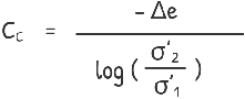
or we can also write it as this

 

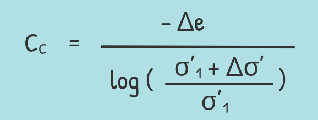
The compression index (Cc) of soil is a crucial indicator of how much a soil sample will compress under increasing pressure. Higher value of compression index indicates a more compressible soil. This characteristic can also be visualized on a graph. As compression index of soil is higher, the curve will be steeper, which means for even a small increase in effective stress, the decrease in void ratio is large. That clearly says the soil is more compressible.

 

 

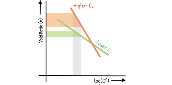
Conversely lower value of compression index represents a less compressible soil, hence the soil is denser and there will be less settlement.

 

So we received lots of information from the curve between void ratio and effective stress. But now one may wonder, that these graphs only represents the increasing value of effective stresses, but while doing the test we also unloaded our sample which reduced the effective stress on soil. Where is that part of the curve?

Well before discussing that part of the curve, we need to learn a little about normally consolidated soil and over consolidated soil and that we are going to discuss in our next post.