Huge mountains and their towering slopes remain standing firm against the forces of nature. What internal strength allows them to withstand these natural forces? This internal strength is a property of the soil known as Shear Strength. We explored Shear Strength and how it's described by the Mohr-Coulomb theory in our previous post.

In short, shear strength is the ability of soil to resist the forces that tend to cause sliding along its internal layers. And that shear strength of the soil is given by Mohr-Coulomb theory as this.

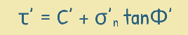
where

• τ’ is the shear stress at failure,

• σ’ is the effective normal stress,

• c is the Effective cohesion between the particles,

• φ is the Effective angle of Shearing Resistance

There are numerous ways to determine the shear strength of soil. In this post, we'll dive into one of the most simple and widely used methods: the Direct Shear Test.

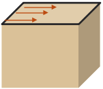
The Direct Shear Test is considered one of the most common and straightforward methods to determine the shear strength of soil. It is a laboratory test, where using machinery, the soil sample is literally sheared across its width, splitting it into two halves along a horizontal plane in the middle. This helps us determine the soil's shear strength.

For the test, the soil specimen is placed inside a shear box. This box is typically made of brass or gunmetal and can be either square or circular in shape. A common size for the square box is 60x60x50 mm. The box comes with grid plates—these are plain for undrained tests and perforated for drained tests.

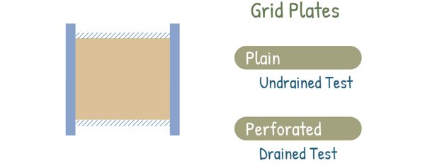
It should be mentioned here that during the test, the soil is compressed, and in the process, water tries to leave the sample. We can either allow the water to escape or drain out of the sample, which is called a drained test, or we can prevent the water from escaping, which is called an undrained test.

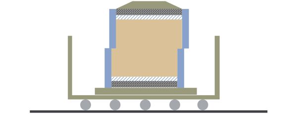
In the setup for drained tests, porous stones are placed at the top and bottom of the soil sample. These stones help water to drain out. To apply the normal load to the sample from the top, a pressure pad is fitted into the box.

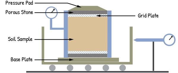
The lower half of the box is securely fixed to a base plate, which is held firmly in place within a larger container. This container is supported on rollers, allowing it to be pushed forward at a constant rate by a geared jack. This setup acts as a strain-controlled device.

A strain-controlled device applies deformation at a constant rate, so the soil sample is sheared at a consistent speed throughout the test. These devices offer high precision and control, making sure the test results are accurate and repeatable.

We track the shear displacement with a dial gauge fitted to the container. To measure the shear force on the soil sample, a proving ring is attached to the system.

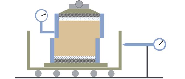
The upper part of the shear box is lifted to create a small gap between the two halves. The size of this gap depends on the maximum particle size in the soil—it's usually kept at about 1 mm.

Now we're ready to start the testing. First, we apply a normal load to the sample to create a normal stress of 25 kN/m². Then, we apply a shear load at a constant strain rate.

The sample begins to shear along the horizontal plane between the two halves. Due to generated forces within the sample, we observe the changes in readings of the proving-ring and dial gauges. These readings are taken every 30 seconds. The test continues until the specimen fails or reaches 20 percent longitudinal displacement, whichever occurs first.

The failure occurs when the proving ring’s readings begin to decrease after reaching a peak. However, there are some soils for which we don’t observe such peak. For such soils we assume that failure has occurred when shearing strain of 20% is reached.

At the end of the test, we remove the sample from the box and determine its water content.

We then repeat the test under different normal stresses of 50, 100, 200, and 400 kN/m². The range of these stresses should cover the typical loading conditions of the field problem we're studying, so we can accurately determine the shear parameters needed.

Before we dive into the results, it's worth mentioning that this test can be performed under any of the three conditions that a soil sample can be tested in. These conditions are:

• UU: Unconsolidated-Undrained, where the sample is not allowed to consolidate or compress and also the water is not allowed to escape during shear process.

• CU: Consolidated-Undrained, where the sample is allowed to consolidate under the normal stress, but water is not allowed to escape during the shear process.

• CD: Consolidated-Drained, where the sample is allowed to consolidate and water is allowed to escape during shear.

Now we begin our calculations with the results of the test. We create a plot of shear stress against shear strain.

To do this, we calculate the shear stress at any point during the test by dividing the shear load, indicated by the proving ring, by the cross-sectional area of the sample.

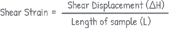
Then, we find the shear strain at a particular load by dividing the shear displacement (ΔH) i.e. is the amount the soil sample moves horizontally during the test, by the initial length of the soil sample in the direction of this movement (L).

Using the data, we plot stress strain curve.

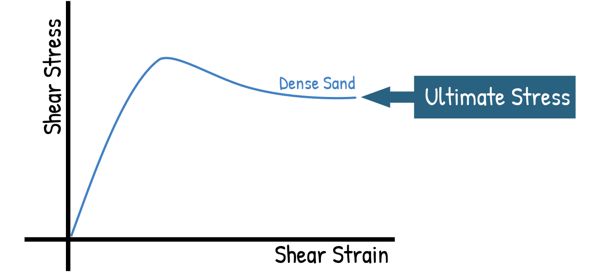
For dense sands, we observe the kind of graph where the shear stress reaches a peak at a small strain. This means the soil can handle a high amount of force in the beginning. But, as the strain keeps increasing, the shear stress decreases slightly and becomes more or less constant, known as the Ultimate Stress. This ultimate stress is important for long-term stability.

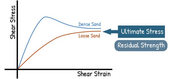
In the case of loose sands, the shear stress increases gradually and then attains a constant value, known as the ultimate stress or residual strength. Interestingly, it's been observed that the ultimate shear stress for both dense and loose sands, when tested under similar conditions, is roughly the same.

We have already seen that the failure of the sample is considered when stress in soil reaches at peak or for some soils which never reaches peak it is, 20% of shearing strain.

With the data obtained from multiple specimens, we determine the shear stress required to cause failure for each normal stress. We then plot all these points on a graph of shear stress vs. normal stress. By connecting these points with a straight line, we get what's called the failure envelope.

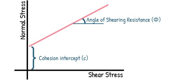
The angle of this envelope from the horizontal gives us the angle of shearing resistance, φ, and its intercept on the vertical axis is equal to the cohesion intercept, c.

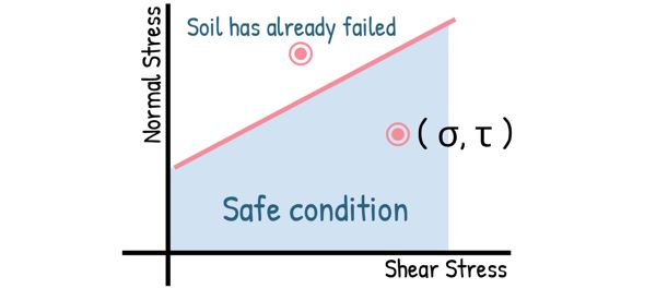
Any point representing a combination of normal stress and shear stress that lies below failure plane indicates a safe condition for the soil. On the other hand, any point above this line represents a condition where the soil has already failed.

The direct shear test is very easy to perform. However, it does have some limitations.

1. When sample is sheared, the stress isn't evenly distributed across the failure plane. Instead, the stresses are higher around the edges, which can cause the soil to fail gradually, almost like how a piece of paper tears. Because of this, the soil's full strength isn't fully utilized all at once across the entire failure plane.

2. the area under shear gradually decreases as the test progresses. Determining the exact corrected area is challenging, so we typically use the original area for calculating stresses.

However, if we do use a corrected area for a more accurate measure of shear stress, the formula is:

A_C = A_O(1 + Δ/3)

A_O = initial area of the specimen in cm

Δ = displacement in cm.

3. We cannot measure the pore water pressure during the test. This is important because pore water pressure affects the effective stress in the soil, which is the stress actually carried by the soil particles.

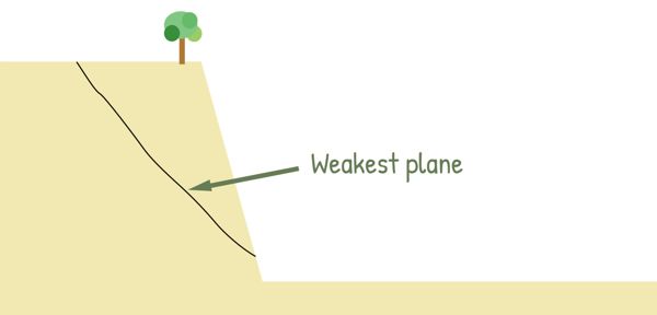
4. The orientation of the failure plane is fixed; it's always horizontal. This might not be the weakest plane in the soil. In real-world conditions, the soil could fail along a different plane that is actually the weakest, so the test might not show the true failure behaviour of the soil.

To address these limitations, the Triaxial test was developed. This test provides a more comprehensive understanding of soil behaviour.