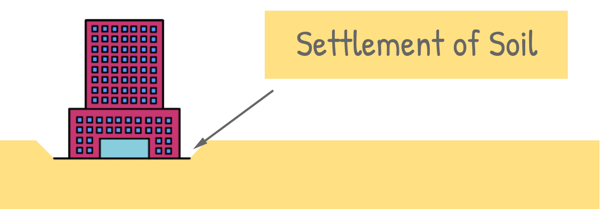
Heavy buildings or structures make the ground compress a little over time due to their weight. This compression of soil is known as the Settlement of soil.

 

 

Total settlement of the soil has primarily three components.

1. Immediate Settlement

2. Consolidation Settlement or Primary Consolidation

3. Creep Settlement or Secondary Consolidation

 

The Total Settlement of soil is the sum of all three factors

 

Consolidation Settlement is the most dominant factor of the total settlement. It refers to the settlement of soil that occurs because applied load causes the rearrangement of soil particles and dissipation of excess pore water pressure in saturated soils. We have learned all this in our previous post.

 

Terzaghi gave a theory that explains the gradual settlement of saturated soils under the application of a load. The theory focuses on the process of expulsion of pore water from the soil voids, leading to a decrease in volume and subsequent settlement.

 

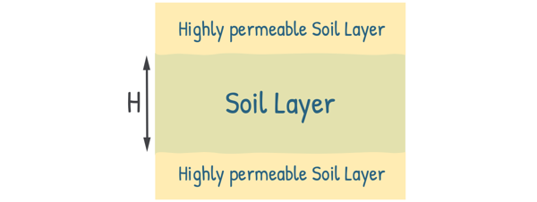
Let us consider a saturated clay layer of thickness H, sandwiched between two layers of sand, meaning the soil layer is surrounded by two highly permeable layers.

 

 

If the soil layer had only the top surface open for drainage and the bottom surface supported by an impermeable rock layer, water could only escape from the top surface. This scenario is known as one-way drainage.

 

 

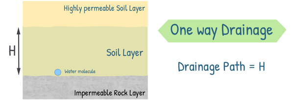
In this case, the water molecules farthest from the open surface would need to travel the entire thickness of the layer, making the drainage path equal to the thickness of the layer, H.

In our system, however, water can escape from either the top or bottom surface, making it a two-way drainage system. The most distant water molecules, located in the middle of the clay layer, only need to travel half the thickness of the layer to reach either permeable boundary.

 

 

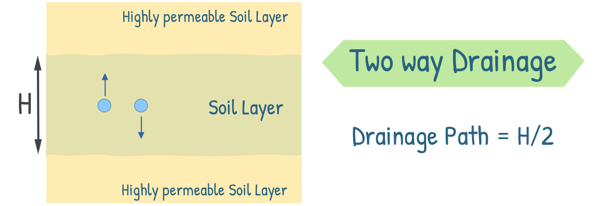
Therefore, the drainage path for water becomes half the thickness of the soil layer, H/2.

 

When we apply a uniform pressure, say Δσ, to the top surface, immediately after the application of the load (at time t = 0), the entire pressure is initially taken up by the water in the soil pore as Excess Hydrostatic Pressure or also known as Excess Pore Water Pressure. This initial excess hydrostatic pressure, say ū_i, is same through out the clay layer.

t = 0,   ū = ū_i

Water begins to escape from the top and bottom of the soil layer, causing the excess pore water pressure at the top and bottom of the clay layer to drop to zero. However, the excess hydrostatic pressure in the middle portion of the clay layer remains high.

t > 0,   ū < ū_i

As consolidation progresses, the excess hydrostatic pressure in the middle of the clay layer decreases and eventually, at time t = tf, the entire excess pore water pressure dissipates. At this point, all the load is supported by the soil particles as effective stress.

t = t_f,   ū = 0

But how does this excess pore water pressure change with time and depth within the clay layer? To analyze this, Terzaghi presented his Consolidation Theory, which describes precisely that.

 

Terzaghi developed his theory to describe the time-dependent settlement of saturated clay layers under applied loads. The theory provides a mathematical relationship between time, settlement, and soil properties. By plotting this relationship, engineers can visualize the consolidation process and make predictions about future settlement.

 

To simplify the analysis, Terzaghi made several assumptions, such that:

1. The soil is homogeneous and isotropic which means soil material is same everywhere and its properties are same in all direction.

2. The soil is fully saturated.

3. The soil particles and water in the voids are incompressible. Hence when the soil is compressed, the consolidation occurs only due to expulsion of water from the voids.

4. Soil is compressed in vertical direction only and with that drainage of water also occurs only in the vertical direction.

5. The time elapsed in the consolidation process entirely depends on the permeability of the soil. This is because, there are other factors also which affects the time of consolidation.

6. The flow of pore water through the soil follows Darcy's law, which states that the flow rate is proportional to the hydraulic gradient and the soil's permeability.

7. Permeability of the soil remains constant during the entire period of consolidation. This assumption significantly simplifies the mathematical equations governing consolidation.

8. The applied load increment causes negligible changes in the thickness of the soil layer. Though the thickness of the soil layer changes due to consolidation, and H becomes (H - ΔH) but  the change in thickness is small enough that the original thickness (H) can be used throughout the consolidation analysis without introducing significant errors. This assumption implies that the coefficients of permeability (k) and volume compressibility (m_v) remain constant during the load increment. Again this assumption is made because it significantly simplifies the mathematical equations that govern consolidation.

 

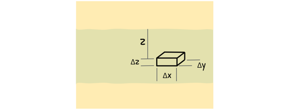
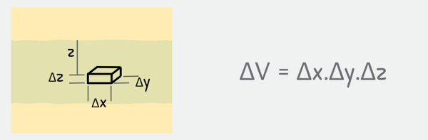
We are not going to derive the entire equation, but we will briefly discuss its derivation. Let's begin with our previous scenario where the clay layer is sandwiched between two permeable sand layers. We consider a small element of thickness Δz at depth z, with other dimensions being Δx and Δy.

 

 

We start with the condition of continuity of flow, which is applicable to all flow situations.

 

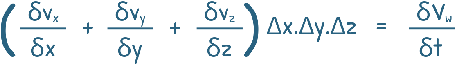
This equation describes the amount of water coming in the soil element minus the amount of water going out of it is equal to the change in the volume of water present inside the element.

As we assumed that only one dimensional flow, in z direction, the equation reduces to this

 

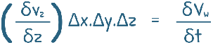
Then next assumption is darcy’s law is valid which says, velocity of water in pores is proportional to hydraulic gradient. And that can be written as this.

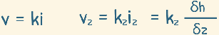
so our equation become 

 

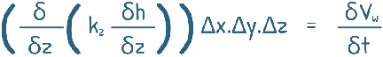
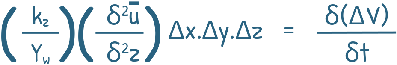
Also one assumption is that soil is homogeneous, hence permeability k_z is not changing and is constant through out depth.

 

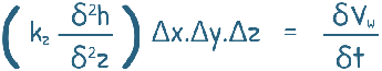
h is the head across the soil element. And this head at any instant and at this particular depth is equal to the Δu/γ_w.

Here Δu is the change in pore water pressure due to applied load, or simply the excess pore water pressure at a particular time. It is also written in different books as ū, u_excess or simply u. We are going to use ū here. Also don’t get confused this ū or u, if it is written, with the pore water pressure. It is excess pore water pressure or change in pore water pressure.

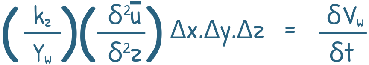
So we can write

 

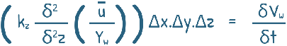
and the equation becomes this

 

Then for the right hand side, which represents the change in the amount of water in the soil element. We should note that change in volume of soil element is actually the change in volume of water, (V = V_w), as solids are assumed incompressible and consolidation occurs only because of water escaping the soil element.

Also in our case volume of soil element is

 

hence we can write change in volume of soil element as this

 

also we know volume compressiblity is defined as this

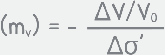
we re-arrange it

and partially differentiate it with respect to time,

 

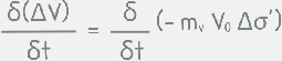
We have also assumed that coefficient of volume compressibility remains constant through out the consolidation process. Also that V₀ is the initial volume of the soil element which is constant. so

 

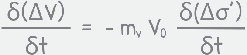
by substituting this in our equation,

 

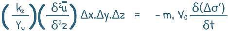
We know at any time t during consolidation the total stress on soil is partly carried by water and partly by solid particles as this

Δσ = Δσ’ + Δu

and for small change in these parameter they become this

δσ = δσ’ + δu

in our case, the total stress is not changing but effective stress and pore water pressure is changing. Hence

0 = δσ’ + δu

δσ’ = - δu

 

so equation arrives at:

 

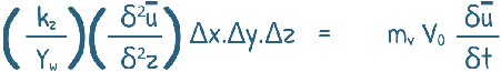
V₀ is the volume of soil element which is equal to ΔxΔyΔz.

Hence this term get cancelled out and we arrive at a neat equation.

 

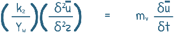
or we can write it as this

 

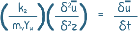
The quantity (k_z/m_vY_w) is defined as the coefficient of consolidation C_V. And our equation is written as this.

 

I think some of you remember this equation very well. The equation highlights the time-dependent nature of soil consolidation, which is important for long-term stability and performance of structures.

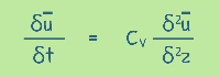
The equation is a form of the diffusion equation, which describes how a quantity, in our case, excess pore water pressure, spreads out over time and space.

The left-hand side of the equation, (δū/δt), represents the rate of change of excess pore water pressure with time. The right-hand side, (δ²u/δz²), shows how the excess pore water pressure changes across different depths in the soil, scaled by the coefficient of consolidation (C_V).

The coefficient of consolidation C_V, controls the rate at which the excess pore water pressure dissipates. A higher C_V, means faster consolidation, while a lower C_V, means slower consolidation. The units of coefficient of consolidation are m²/s or m²/day.

C_V is not a constant, but while both permeability (k) and volume compressibility (m_v) tend to decrease as soil compresses, their combined effect on the coefficient of consolidation (C_V) often results in relatively stable values across a reasonable range of pressures.

 

The solution of this basic differential equation {(δū/δt) = C_V(δ²u/δz²)} is very simple. All we have to use is Fourier series and some boundary conditions. I guess that problem is enough for a life time.

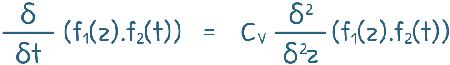
So, we won’t go deep but would look at the overview to get a better understanding. For the solution of the this equation, we begin with considering excess pore water pressure ū as a function of depth and time.

ū = f₁(z).f₂(t)

 

Then putting it in the equation:

 

When we solve this equation we arrive at solution where we need to get some values of the quantities, and for that we use boundary conditions.

 

Let us state the boundary conditions.

(i) At time t = 0, that is, just after the application of load on soil, the excess pore water pressure is same at any depth in the soil and is equal, say ū_i. And this ū_i is equal to Δσ, as we know all the pressure at the beginning is supported by water only.

At t = 0 , ū = ū_i , for any value of z

 

(ii) at t = ∞, the excess pore water pressure is zero everywhere, as the consolidation is considered as compelete.

At t = ∞ , ū = 0 , for any value of z

 

(iii) At any time after the application of load, at the top surface of the clay layer, i.e. at z =0 , the excess pore water pressure is zero.

At t > 0 , ū = 0 , z = 0

(iv) At any time after the application of load, at the bottom surface of the clay layer, i.e at z = H, the excess pore water pressure u is zero.

At t > 0 , ū = 0 , z = H or 2d

(we can also write depth z as twice of drainage path in case of 2 way drainage)

 

Then by further solving the equation by applying the boundary conditions, we arrive at this equation.

 

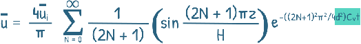
In this equation, the quantity ( C_vt/d²) is defined as the Time Factor T_V.

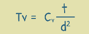
It is a dimensionless quantity. We will talk about it a little later in this post.

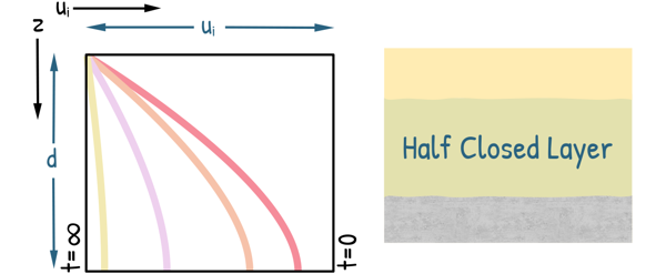
The solution to Terzaghi's one-dimensional consolidation equation can be visually represented through a plot illustrating the variation of excess pore water pressure with depth and time. Multiple curves are plotted, each representing a different time interval. The relative positions of these curves depict the dissipation of excess pore water pressure over time.

 

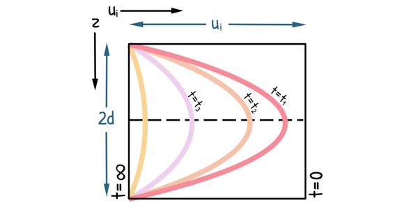
Key observations from the diagram:

We can observe that Immediately after load application (t=0) the initial curve is a vertical line, indicating maximum and uniform excess pore pressure throughout the soil layer.

As time progresses (t>0), excess pore water starts to dissipate, and the curve become parabolic in shape. The highest excess pore pressure is observed at the midpoint of the consolidating layer, gradually decreasing towards the drainage boundaries.

With further consolidation, the curve flatten out and move closer to the zero excess pore pressure line. Eventually, when the curve becomes a vertical line, the excess pore pressure has completely dissipated, and consolidation is complete.

 

The shape of this curve also depends upon the drainage conditions at the boundaries of clay layer. If both the upper and lower boundaries are free draining, the clay layer is known as open layer and shape of the curve will be parabolic.

 

 

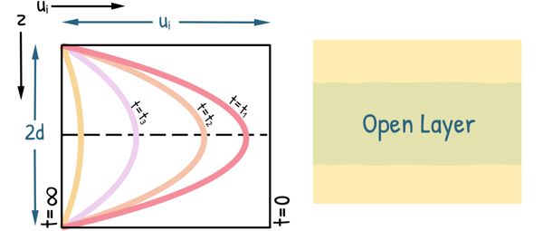
If only one boundary of the clay layer is free draining, the layer is called a half-closed layer, and the shape of the curve is a half-parabola.

 

 

 

Terzaghi also introduced the concept of the Degree of Consolidation (U).

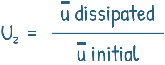
At any point at depth z, the degree of consolidation U_z, is the ratio of the excess pore water pressure that has been dissipated at that point to the initial excess pore water pressure at that depth.

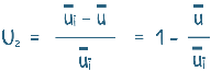
Excess pore water pressure dissipated can be written as initial excess pore water pressure minus the excess pore water pressure present at that point at any given time.

 

it can also be written as this.

 

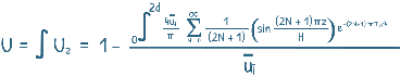
This equation gives Degree of Consolidation at any depth, but we are more interested in knowing the average Degree of Consolidation of the whole layer.

So, if we substitute that massive equation and integrate it for the whole depth of the soil, we find that the average degree of consolidation U is dependent on the non-dimensional time factor T_V.

U = f(T_V)

 

The time factor allows engineers to estimate the degree of consolidation at any given time. The relationship between Time factor and Degree of Consolidation can be summed up into the following empirical formulas.

Tv = (Π/4) U2 (for U ≤ 0.60)

Tv = -0.933 log₁₀(1-U) – 0.085 (for U > 0.60)

 

By knowing the value of coefficient of consolidation, C_V, we can estimate the time required for a given percentage of settlement to occur. For example, If we want to estimate the time required for a soil layer to achieve 80% consolidation, we can use the above equations to calculate the time factor. Then, using the equation Tv?=C_V(t/d²), we can calculate the actual time required (t).

 

This Consolidation analysis made by Terzaghi is very simple, but it is based on assumptions that are not practical in real-world situations. Hence, there are a number of limitations to the theory.

1. We considered the soil to be homogeneous and isotropic, which is not the case in the field.

2. We assumed that the solid particles and water in the voids are incompressible. However, in reality, solid particles do compress, which is the cause of secondary consolidation in soil.

3. We assumed that the soil is compressed only in the vertical direction and that drainage of water also occurs only in the vertical direction. However, in actual situations, water drainage and soil compression occur in three dimensions.

4. We also ignored the initial and the secondary consolidation in this analysis.

5. The load on the soil is not usually applied all at once. It takes sometime to build any structure. So load is gradually increased on the soil.

6. We assumed that the change in thickness of the soil layer due to the applied load increment is negligible and it was not considered. Additionally, permeability and the coefficient of volume compressibility are considered as constant, while their values change with the load increment.