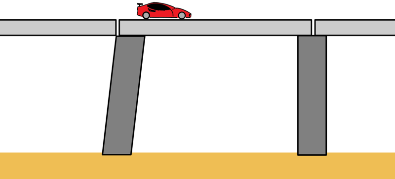
When we think of engineering failures, we usually imagine dramatic catastrophes — a bridge snapping in half, a building collapsing into dust or a fan blade suddenly flying out of a jet engine.

We think about things breaking.
In engineering, we call that a Strength failure. And yes, we obviously design things so they don’t break.
But there is a another type of failure that is less dramatic and much more silent and common. It’s called a Serviceability failure. That is, the structure or component loses its service capabilities for which it was designed.
In serviceability failure, a structure may be perfectly safe and perhaps nowhere near breaking, but it bends, moves or deforms so much that it becomes uncomfortable, unreliable, or even unusable.
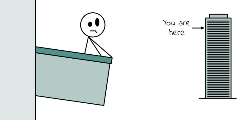
Imagine standing on a balcony on 40th floor of a high-rise. We have been assured by engineers that this balcony won’t break. But we see it has tilted visibly down to a steep angle. Anybody going to stay there? Absolutely not.
Or think about a rotating shaft with gears mounted on it. Even a tiny deflection can misalign the gears, leading to uneven contact and excessive wear over time.
So engineers don’t just design for strength — they also design for how a structure behaves in use.
That bending — whether it’s in a shaft or a balcony —
is usually measured using just two things.
1. Deflection — which is how much a beam or any other component moves vertically up or down.
2. Slope — which is the angle it makes as it tilts.
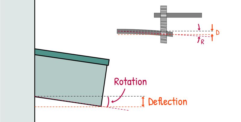
To prevent a strength failure, we calculate stress. To prevent a serviceability failure, we calculate Slope and Deflection.
So , how do we actually find these? How do we predict how much a beam will sag, and how much it will tilt, even before we build it?
Quick Note : To make things easier, I’ve collected all the important formulas of Strength of Materials into one Formula sheet — you can check it below if you need it.
Let’s start with a simple case of a straight horizontal cantilever beam.
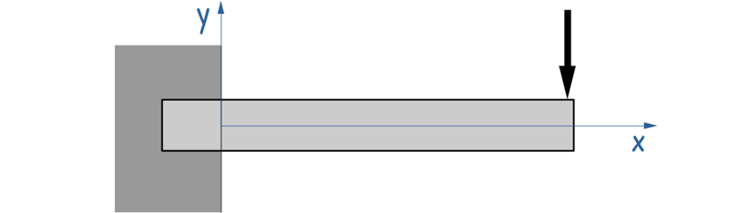
We define an x-axis along the length of the beam, positive to the right. And a y-axis positive vertically upward, which will measure how much the beam deflects.
Now when loads act on this beam, they create bending moment inside it and that tries to curve the beam.
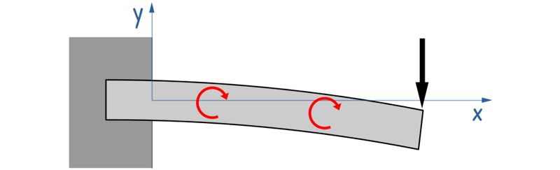
If the moment is small, the beam bends slightly. If the moment is large, the beam bends more.
As the beam bends, it forms a smooth curve. To describe how ‘sharp’ this bending is at any given point, we use the term curvature. We will talk about this curvature a little later in this post.
At this initial stage, it is often helpful to sketch the deflected shape of the beam. This gives us a visual sense of how it bends, and helps us check whether our final answers make physical sense.
This deflected shape is called the elastic curve of the beam.
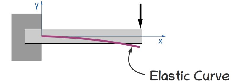
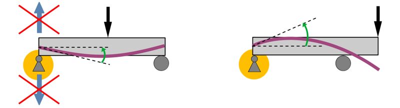
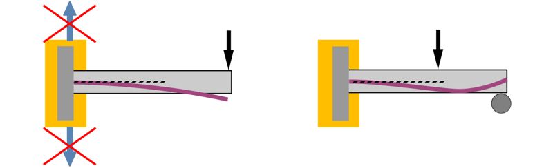
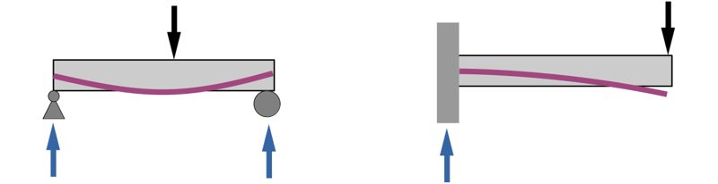
For most cases, the elastic curve can be sketched without much difficulty. However, while doing so, we must pay attention to the type of supports, since they restrict how the beam can move.
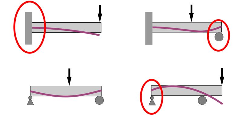
A roller support restricts vertical displacement but allows rotation.
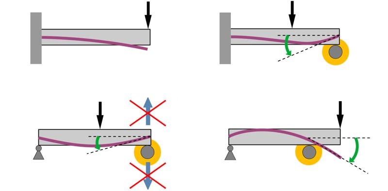
A pin support behaves similarly — it prevents vertical movement and allows the beam to rotate.
A fixed support, on the other hand, prevents both vertical displacement and rotation.
If the elastic curve for a beam seems difficult to establish, we can use the bending moment diagram to guide us. We first draw the moment diagram for the beam. If we use the standard sign convention, a positive internal moment tends to bend the beam concave upward. Likewise, a negative moment tends to bend the beam concave downward.
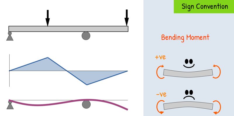
By combining these two facts — the physical restrictions of the supports and the direction of the bending moments, we can sketch a reasonable shape of the beam’s elastic curve.
Now, back to our cantilever beam. Mathematically, the equation of this elastic curve or elastic curve for any beam can be expressed as y = f(x).
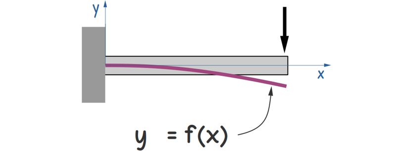
At any distance x from the origin, the function gives us the corresponding value of y and that value gives the deflection of the beam at that point. This deflection is represented as Δ.
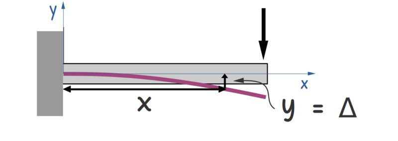
If we differentiate this equation with respect to x, we get dy/dx. It simply tells us — as x changes, y changes.
And the rate of that change is what we call the slope of the curve. This slope is the physical rotation of the beam at that exact point.
Now, mathematically, the slope is equal to tanθ. But for very small rotations, tanθ is approximately equal to θ.
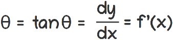
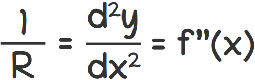
If we differentiate once again, we get d²y/dx². This quantity represents how rapidly the slope is changing, and therefore how sharply the beam is bending.
It is not exactly the curvature, but for the small deflections we usually deal with in engineering, it is a very good approximation.
… (1)
Here,
R is the radius of curvature,
and 1/R represents the curvature.
To build some intuition about the curvature, think of a small circle. It has a little radius, but it is very curved so its curvature is high.
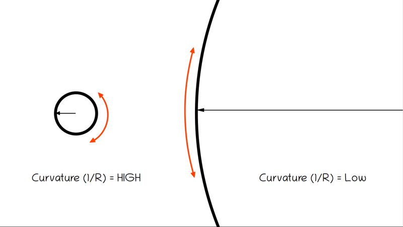
Now think of a very large circle. It has a huge radius, but it is barely curved, it looks almost flat — meaning its curvature is very small.
So far, we have developed the mathematical description of the beam’s shape. Now let’s look at the physical side.
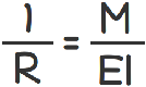
For a beam, how much it curves at any point depends on three factors:
- How hard the load is trying to bend it, that is the bending moment acting at that point, M(x)
- What it’s made of, that is the material stiffness or young’s modulus E
- Its cross-sectional shape which offers geometric stiffness, and that is represented by the moment of inertia, I
There exists a relationship between these quantities and the curvature of the beam, given by:
…(2)
Now, combining equation (1) and equation (2), we get:
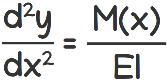
Keep in mind that the bending moment varies along the length of the beam, so it is a function of x, whereas E and I are usually constant for a given beam.
It tells us that the curvature and hence the shape of the beam at any point is directly governed by the bending moment at that point.

Once we know the moment function M(x), we can build the shape step by step through integration.
If we integrate this new equation, we get dy/dx which represents the slope or rotation of the beam.
And when we integrate it second time we get the y , which represents the deflection of the beam at any point.

Also from the known basic equilibrium relationships, we know
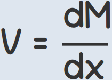
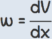
so, we can write two more differential equations in terms of shear force and loading on the beam :
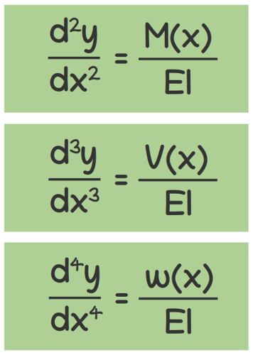
To determine the deflection y, we solve these equations by successive integration. Each integration introduces a constant of integration.
If we start from the load equation and integrate four times, we will have four constants C1, C2, C3 and C4.
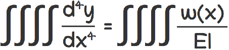

To find the actual values of these constants, we have to look at specific, known physical points on the beam where the shear, moment, slope, or displacement are already completely obvious to us. These known values are called boundary conditions.
For example:
At simple supports, the deflection is zero.
At a fixed support, both deflection and slope are zero
Once all constants are determined, we obtain the complete equation of the elastic curve. This equation allows us to find the deflection y at any point along the beam, at a distance x from the origin.
Let’s find the equation of the elastic curve for our example beam.
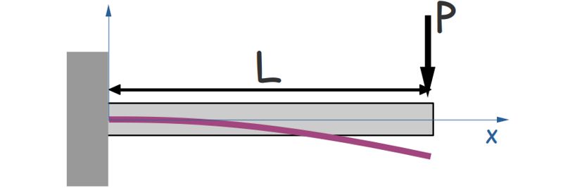
Let’s say length of this cantilever beam is L and the point load pushing down on its free right end is P.
First, we sketch our expected deflected shape. We know the wall will hold the beam perfectly flat at the start, and it will gently curve downwards towards the free tip.
For this case, it’s easier to determine the bending moment equation, so we start with this equation.
Now, let’s find the bending moment at a section located at a distance x from the fixed end:
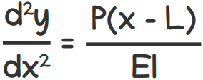
M(x) = P(x – L)
we substitute this in our curvature equation.
now we integrate it once

This gives us the slope or rotation of the beam at any point.
Now we integrate it second time.

and this is the deflection.
Now to find these constants C1 and C2 we apply boundary conditions.
Our beam is fixed at one end. At fixed support the rotation of the beam is zero.
So at x = 0, dy/dx = 0
dy/dx = P/EI ((0)2/2) – L(0) + C1 = 0
this gives us
C1 = 0
Also at fixed support beam cannot displace vertically so deflection (y) is zero at x = 0
y = P/EI ((0)3/6) – L(0)2/2 + (0)x + C2 = 0
and this gives us
C2 = 0
So finally the equation of elastic curve become
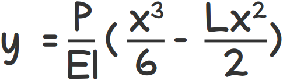
Using this equation, we can find the deflection at any point along the beam. For example at the free end, that is at x = L, the deflection is
y = P/EI (L3/6 – L(L)2/2)
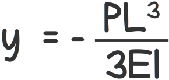
This negative sign acts as a physical reality check. It tells us that the deflection is acting in the negative y-direction—meaning the beam is physically sagging downwards, exactly as we sketched at the start.
For the solution of this problem we started with the moment equation. The choice of which equation to start with depends on the problem. In most cases, however, it is more convenient to first determine the internal moment M as a function of x, then integrate it twice to obtain the slope and deflection. This approach reduces the number of integration constants to be evaluated.
Now, everything we’ve done so far works nicely when the loading is simple. But what if the loading is a bit more complex — like a mix of point loads and distributed loads?
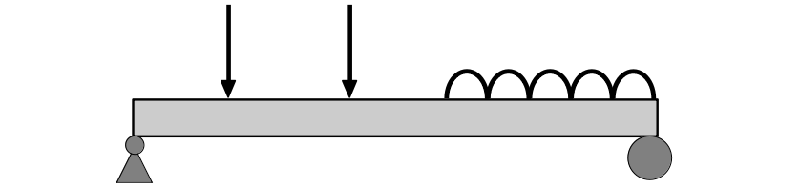
In that case, one single equation for bending moment won’t work for the entire beam. So what we do is, we divide the beam into smaller sections. Each section then has its own bending moment equation.
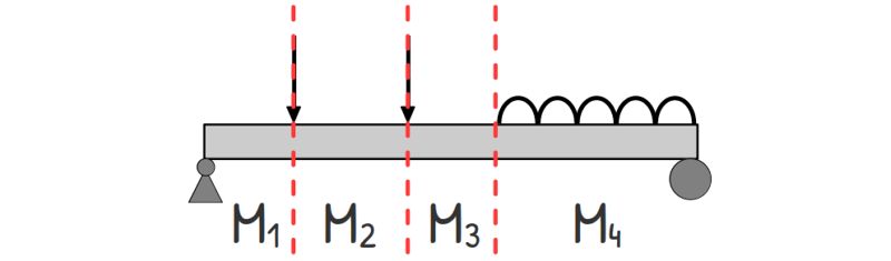
The important thing to understand is that even though we’ve divided the beam into sections, it is still one continuous piece. That means the beam cannot suddenly break or form a sharp corner at the junction between two sections. So both the deflection and the slope must remain continuous. In other words, the deflection and slope at the end of one section must be equal to the deflection and slope at the beginning of the next section.
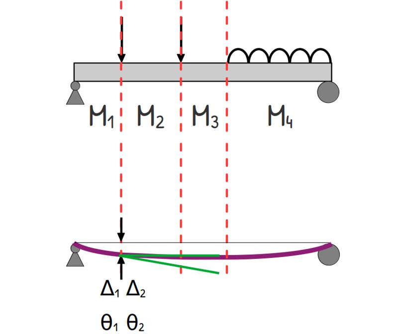
These are called continuity conditions, and we use them along with the boundary conditions to determine the remaining constants of integration.
This is just one of the many methods used to find the slope and deflection of beams. In the coming posts, we’ll explore some other methods as well.
If this post was helpful, here is the link to the formula sheet where all the important formulas are in one place.