A soil mass is composed of small solid particles which we call the soil grains. These soil grains when depositing in a soil mass arranges themselves in a way that some amount of empty space is enclosed between them. We call these spaces voids. Water can flow though these voids.

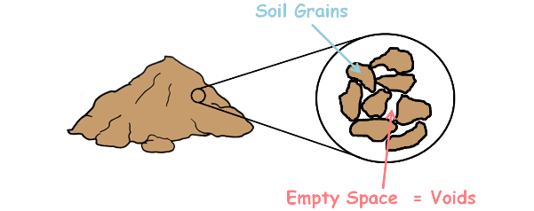
The property of the soil which it permits the water or any liquid to flow through it through its voids is called permeability. Permeability is the ease with which water can flow through the soils.

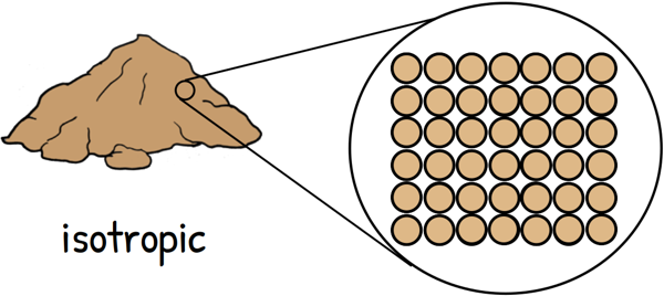
If soil consisted of perfectly spherical grains and if those grains are arranged perfectly in a particular fashion through out the soil mass then properties of soil like permeability will be same in all directions and we say that soil is isotropic.

But in reality soil doesn’t consist of perfectly spherical grains nor they are perfectly arranged in any particular fashion. They are irregular, angular, flaky or elongated. Hence they encloses irregular channels of voids in different directions causing the properties of the soil different in different directions. A material, properties of which are dependent on the direction, is referred to as anisotropic.

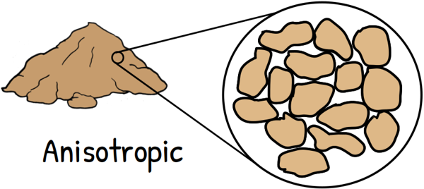
In an inhomogeneous soil deposit water faces different movement resistances when it moves in different directions as the soil has different types of variations in different directions. Consequently we observe different values of permeability in different directions.

Isotropic means having identical values of a property in all directions and anisotropic means different properties in different directions.

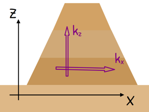
In an earth dam embankment soil has been compacted in layers. There is always some difference in permeability in horizontal and vertical directions. In such anisotropic soil if these directions are denoted by x and z respectively, then we can write permeability in x direction as k_x and permeability in z direction as k_z.

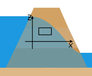
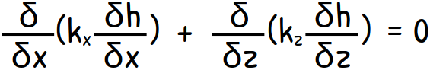
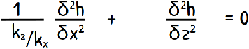
If we are to analyse the fluid flow through this soil, let us consider a soil element through which water is percolating. For the 2-dimensional fluid flow through this element the equation of continuity can be written as this

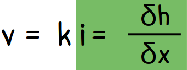
if we assume Darcy’s law is valid which means soil element is fully saturated and flow in the voids is laminar then we can write velocity of fluid is equal to permeability of the soil element times the hydraulic gradient across this element.

v = ki

Hydraulic gradient across this element is given as this

substituting this into the continuity equation

and solving it we get

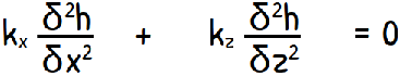.................................( equation 1 )

If the soil had been isotropic then its permeability in x direction and z direction would have been equal

(k_x = k_z = k)

and the equation would have become a Laplace equation.

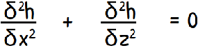.............................. (Laplace Equation)

Laplace equation describes the loss of energy through the space and in our case that energy is in the form of hydraulic head.

When we solve a Laplace equation we receive two families of curves. One set of curves is known as flow lines and other set is equipotential lines. Once we get these lines, we may be able to obtain a graphical solution to the Laplace equation and that is called flow net. Using that flow net we may calculate our desired quantities like seepage through soil.

But our soil is not isotropic and its anisotropic. If we are, somehow, able to convert our equation number 1 into a Laplace equation, we may find the quantity of seepage through the soil of an earth dam with anisotropic properties. So to bring Laplace equation out of that equation we have to modify some elements in that equation.

Lets divide the equation by k_z

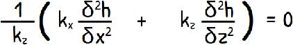
re-arranging it a little...

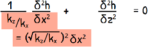
and we write highlighted part of the equation as the following

re-writing it...

--------------------------- (equation 2)

Now this equation looks little be similar to Laplace equation. Only highlighted part is problematic.

Now let us use our creativity and out of nowhere this thought comes into our mind that why not write

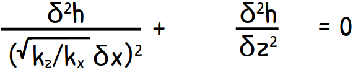
and when we partially differentiate it with respect to x, we get our problematic term.

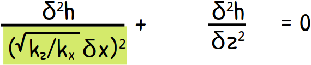
so lets substitute this in our equation number 2 and with it the equation becomes the Laplace equation in x_t-z plane.

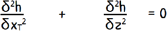
This is also a continuity equation for an isotropic soil in a fictitious x_t-z plane.

What we did here is, we transformed the anisotropic soil medium, medium which has different properties in different directions, we transformed it by scale transformation in the x direction to obtain isotropic medium, which has similar properties in different directions and for which the Laplace equation is valid. We did so as to construct the flow net and find solutions to our engineering problems in anisotropic soil.

Now, for this new transformed section we can draw the flow net by following the method of constructing the flow net.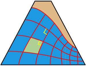

As we have transformed this section to isotropic the flow net for this section will have orthogonal intersections of flow lines and equipotential lines with all its fields being elementary elementary squares.

Consider a flow field in the flow net across which the flow is taking place and let us show it as normal square for simplicity. The natural flow field is elongated but we have transformed it to a perfect square.

For the natural elongated section the coefficient of permeability in the horizontal direction is k_x and in vertical direction is k_z. While in transformed square section the coefficient of permeability is, say, k’ in both x and z directions because now the soil is isotropic and it has similar properties in both the directions.

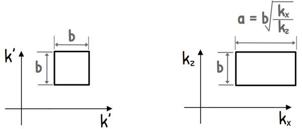
lets say length and height of this elementary square is small b and that of natural flow field is a and b. we know a has been transformed into b so we can write a as square root of (kx/kz)) times b because if we remember we transformed the section this way only.

Since both are same sections, the quantity of water that flows through the section in both cases must be equal. So we can write quantity of water Q is equal to permeability of this section in this direction multiply by the cross-section area A multiplied by hydraulic gradient across this section i.

Q = kAi

Permeability in x direction is k’ and k_x for the respective sections. Area of the flow is height b and width lets say y.

Q = kAi = k’ (b.y) i = k_x (b.y) i

and If ΔH is the head loss across the field

so hydraulic gradient in elementary square is ΔH/b and in the natural flow field ΔH/b√(kx/kz).

solving this we get the effective coefficient of permeability applicable for our transformed section.

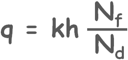
Now, that we have effective permeability of the transformed section, using the flow net the seepage quantity q can be computed from the equation that we have discussed in the flow net article.

Though the flow net on the transformed section does not present the correct picture of flow pattern. The true flow net can be drawn by re-transforming the section back to its original dimensions. On the natural cross-section, the flow net will not be composed of squares because the horizontal dimensions are elongated by the factor √(kx/kz), nor will there be orthogonal intersection between the flow lines and the equipotential lines.